A theoretical physicist's dictionary for machine learning, starting where both fields start: statistical mechanics, maximum entropy, and why the Boltzmann distribution is the most likely one.
By Mirco Milletari · January 13, 2020
Intro
I have been trained as a theoretical physicist, working on complex quantum systems. Since I moved in the machine learning business, I couldn't stop noticing how much this field share with the physics I have been using for long time. This is not accidental if you consider that physicists have been interested in solving complex optimization problems for quite a long time, especially in relation to a class of systems called spin-glasses; these systems share some of the features of Neural Networks, in particular a complex Loss landscape with many metastable minima. The mathematical concepts developed to understand Spin Glasses and other complex systems are so fascinating and so general that physicists have used them to study the performance of classical optimization problems in computer science, such as minimum-cut, minimum-cost, graph-coloring, satisfability etc... However, the language used by physicists is often very different than the one used by computer scientists, making it difficult to share ideas. Often, during my short career in machine learning, people asked me: what has physics to do with machine learning... my answer is: a lot! This blog is for those who do not see this connection or that are just curious to know more about how the two fields are interconnected.
In this blog series I will try to create a sort of dictionary for physicists who want explore Neural Networks and for computer scientists/engineers who are interested in understanding how physicists try to understand these models. There is no better way of doing that than showing how things are done in details. So the content of this blog will be somehow technical, but hopefully still clear. When showing the math, I will follow the physicist's way of getting numbers out of a calculation, rather than bounds and/or theorems. When analyzing the performance of an algorithm, computer scientists often look at worst/best case scenarios while phycisists are interested in the typical ones. For example, the outcome of each indivisual experiment may be slightly different everytime we collect the data (this is especially true in quantum systems), either for intrisic or extrinsic reasons. Phycisits are usually interested in calculating the most likely outcome rather than the worst/best one, that is usually understood as a large deviation event. A physics model returns a "number", a clear prediction that experimentalists can either verify or prove wrong. In my opinion (and yes I am biased) this a more useful viewpoint when working in machine learning: a Theoretical model giving a "number" we can compare to the numerical outcome.
Before getting into the details of how these different models are built and their meaning, let me use this first post to introduce the framework I will use, a theory called Statistical Mechanics (SM). This theory was introduced towards the end of the 19th century in order to reconcile the laws of thermodynmics and the "newly" proposed atomistic view of nature. Scientists like Boltzmann, Gibbs etc.. contributed to lay the foundations of this framework that proved very effective to explain the macroscopic world starting from its smaller constituents. The theory was later provided with solid mathematical foundations that I will not discuss here; the interested reader can see e.g. []. Also, I will discuss how this theory is at the basis of information theory and hence several concepts in computer science.
Statistical Mechanics for pedestrians
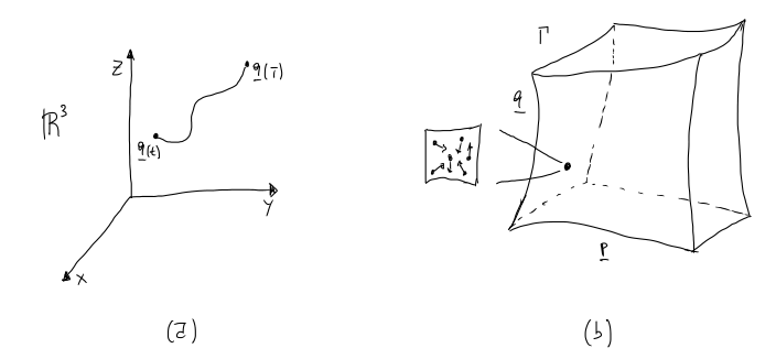
The aim of Statistical Mechanics (SM) is to obtain the macroscopic behaviour of a system starting from its microscopic constituents. By the end of the 19th century phycists had a good understanding of the laws of thermodynmics, expressed by simple equations relating different measurable quantities, e.g. 𝑃𝑉=𝑛𝑅𝑇 relates pressure (P), volume (V), temperature (T) and moles number (n) via a constant (R). Boltzmann embraced the old atomistic idea, dating back to Democritos (!), that all matter is composed of elementary building blocks, particles moving and interacting. If these particles existed, and this was not the common view at the time, they had to follow the "universal" laws of dynamics layed down by Newton some time before. So how can you describe a gas and its properties starting from particles moving around? In the Hamiltonian formalism of mechanics [], we need to specify two vectors for each particles we want to follow: momentum and position. You may recall that momentum 𝐩=𝑚𝐯 is mass times velocity and position 𝐪; these are also known as generalized coordinates. So momentum and position uniquely define (at least in classical mechanics) the status of a particle at some time 𝑡. We are used to visualize the position of an object in a plot; to be more specific, let us work in three dimenions so that the position of our particle can be represented as a point in a cartesian space with axes 𝑥,𝑦,𝑧. As the particle moves, it traces a trajectory in this space, parametrized by time, and defined by 𝐪(𝑡). We can abstract this construction to represent both 𝐩(𝑡) and 𝐪(𝑡) in a space; for 𝑁 particles such a space has 2𝑑𝑁 dimensions (6𝑁 if each particle has 3 degrees of freedom), see Fig. (1).
Figure 1. (a) Particle’s trajectory in the three dimensional position space, 𝑇>𝑡. (b) A schematic representation of the 2𝑑𝑁-dimensional phase space manifold Γ. A single representative point in Γ represents the status of the entire system at some time 𝑡. The inset represents a cartoonish zoom in the representative point, where particles’s positions and their momentum (arrows) are schematically represented.
We call this space, the phase space and denote it as Γ. A single point in Γ represents the status of the system at time 𝑡, for this reason it is often called a representative point. In principle, one could determine the evolution of the system in time by solving the equation of motions for the 𝑁 particles. How many particles are in a gas or in a general macroscopic system? You may recall Avogadro's number: for each mole there are 1023 particles, so we should be able to solve a comparable number of differential equations, a task that was not only impossible at the time of Boltzmann, but also on modern supercomputer! However, as we discussed above, thermodynmics is governed only by a small number of parameters, so how do we recondile these two approaches? Clearly, not all the information encoded in those 6𝑁 degrees of freedom per second is relevant. As the macroscopic world emerges from the microscopic, only a small number of coarse grained quantities are relevant, e.g. temperature is the average kinetic energy of the particles, pressure is the average force the particles in a gas exert on the wall of the container etc... The idea at the very foundation of Gibbs' approach is to replace an average over time with a distributional average called ensemble average. The problem obviously is: how do we choose such a distribution on Γ? To answer this question we need to introduce the theory of Statistical ensembles; instead of doing this the traditional way [1, 2], here I want to show you a more modern approach inroduced by Jaynes [3, 4] that has the advantage of making the connection to information theory and other concepts in machine learning quite simple.
Ensemble measure from Maximum Entropy
Let us start by introducing an important concept you may be already familiar with: the Entropy. If you are coming from a machine learning background, you have probably used the cross-entropy loss to train your classifier, here I want to show you where this quantity comes from and how it "leaked" in computer science. Boltzmann defined the entropy of a system as:
𝑆=𝑘𝐵log𝑊,(1)
where 𝑊 is the volume in phase sapce accessible to the system and 𝑘𝐵 is a constant with dimension of energy times inverse temperature. The natural logarithm is counting the number of configurations corresponding to a macroscopic state. Well, this may sound a bit cryptical, but it will be clear in a shortwhile; before getting into the math, in plain english it means that many different microscopic configurations of a system correspond to the same macroscopic, observed one. Take the temperature for example; you may recall that I have stated without proof that it corresponds to the average kitetic energy of the N particles in the system. The point is that this definition does not care about the kinetic energy of the single particles, say particle 𝑝1 has energy 𝜖1, particle 𝑝2𝜖2 etc ... we could swap the labels and say that 𝑝1 has energy 𝜖2 and 𝑝2 energy 𝜖1, the mean energy ¯𝜖=(𝜖1+𝜖2)/2 is the same for these two different configurations. However, we could prepare the system in a very special configuration; this configuration will occupy only a specific point in phase space, for which 𝑊=1 and therefore 𝑆=0; this state is so special that it is unlikely to happen spontaneouly. On the other hand, most likely states, correspond to those with higher entropy, i.e. those configurations that occupy a larger volume of the phase space (I'll come back on this in a moment). The other interesting property of 𝑆 is that it is an "extensive" quantity, i.e. the entropy of two systems is the sum of the entropies of the two single systems. Enough with talking, let us get to the math!
Let us follow [1, 2, 3, 4] and find which is the most probable distribution on Γ. As we define spaces of "numbers", and functions mapping one number into another, we can define space of functions and "functionals", mapping functions into functions, see e.g. Ref. [5] for a quick introduction to functional calculus, or Ref [6] for a comprehensive one. In this space of all possible distributions, we want to find the one that maximizes the entropy on Γ, i.e. the distribution that occupies the largest volume in Γ.
Let us start by dividing the phase space in 𝑀 cells; according to our previous discussion on the number of degrees of freedom in phase space, you can see that the infinitesimal volume element is 𝑑Ω=∏𝑖𝑑𝐩𝑖𝑑𝐪𝑖=𝑑𝑝𝑑𝑁𝑑𝑞𝑑𝑁, so that each particle occupies 𝑑𝑝𝑑𝑑𝑞𝑑. We devide the phase space volume is smaller, but finite elementd 𝜔𝑖,𝑖=1,...,𝑀, each volume element occupied by a certain number 𝑛𝑖 of particles, also knonwn as "occupation numbers". For every cell 𝑖 we can specify the average kinetic energy of the 𝑛𝑖 particles, 𝜖𝑖=𝐩2𝑖/2𝑚. Specifiying a distribution function on Γ means specifying how the 𝑁 particles are distributedin the 𝑀 cells. The way we divide the phase space volume should be completely irrelevant to the end of getting the correct macroscopic observables; if any cell were special, then our results would depend on the way that we partition the phase space. From now on, we take all 𝜔s to be the same and drop the index 𝑖1. As a consequence, each box has an equal probability of containing a particle, with probability 𝑓𝑖=𝑛𝑖/𝜔. Finally, we enforce two macroscopic contraints:
𝑀∑𝑖=1𝑛𝑖=𝑁,𝑀∑𝑖=1𝜖𝑖𝑛𝑖=𝐸.(2)
The first condition enforces particle number conservation, while the second energy conservation, where 𝐸 is the total energy of the macroscopic system. Note that the latter condition also assumes that the system is "diluted", i.e. interactions play little to no role. For the sake of correctness let me say here that interactions between particles do play a big role to bring the system towards to equilibrium however, once equilibrium is reached, they are no longer necessary to describe this state. If this sounds confusing to you do not despair! It took people quite a long time to accept it; the precise mathematical formulation of this statement was given by Boltzmann in his H-theorem, see [1, 2] if you are curious. Going back to our task we now ask: Which portion 𝑊 of the entire phase space Γ is occupied by the system? Fix a specific configuration for the moment; one particle occupies a volume 𝜔, then 2 particles will occupy a phase space volume of 𝜔2 (see again how the N-particle volume element was defined above) so 𝑛𝑖 particles will take 𝜔𝑛𝑖. As we want to consider the volume occupied by all possible configurations, we need to include a combinatorial factor. In how many ways can we place 𝑁 distinct particles into 𝑀 distinct cells, with 𝑛1 particles in the first cell, 𝑛2 in the second, etc. ? Well, this number is given by the multinomial coefficient, and we find that the phase space volume can be written as:
𝑊=𝑁!∏𝑖𝑛𝑖!∏𝑖𝜔𝑛𝑖.(3)
In case you got a bit lost let me summarize what we have done so far before getting into the math. We want to find the distribution that occupies the largest phase space volume 𝑊. In order to do so, we discretize the phase space in smaller (but finite) cells 𝜔 and fill them with (non-interacting) particles satifying the macroscopic conditions in Eq. (2). We now proceed maximizing the entropy (1); in order to enforce the macroscopic constraints we use the method of Lagrange multipliers [6], and build a new functional (here we use 𝑘𝐵=1 and reinstate at the end of the calculation):
F[𝑛𝑖]=log𝑊[𝑛𝑖]−𝛼(∑𝑖𝑛𝑖−𝑁)−𝛽(∑𝑖𝑛𝑖𝜖𝑖−𝐸).(4)
Our working assumption is that the 𝑀 cells are populated by a large number 𝑛𝑖 of particles and 𝑁≫𝑀; this allows us to use Stirling's approximation for the factorial 𝑁!≃√2𝜋𝑁𝑁𝑁𝑒−𝑁 for 𝑁≫1, see e.g. appendix B in Ref. [2] for a nice derivation of this result. Using this approximation in the entropy and retaining only the leading terms we obtain:
log𝑊[𝑛𝑖]≃𝑁log𝑁−∑𝑖𝑛𝑖log𝑛𝑖𝜔.(5)
We are now ready to maximize the functional defined in (4) by varying 𝑛𝑖→𝑛𝑖+𝛿𝑛𝑖 (where 𝛿𝑛𝑖≪𝑛𝑖), and keeping terms up to the second order in the variation. The linear terms are trivial; the term involving the logarithm can be written as
The optima is obtained from the condition that the first functional variation is zero, while the sign of the second variation tells us if this is a maximum or a minimum (or a saddle):
𝛿F=0→¯𝑓𝑖=¯𝑛𝑖𝜔=𝑒−𝜇𝑒−𝛽𝜖𝑖𝛿2F=−∑𝑖𝛿𝑛𝑖12𝑛𝑖𝛿𝑛𝑖<0,(8)
where 𝜇=1+𝛼 is a constant to be determined, ¯𝑓𝑖 the most likely distribution; since the second variation is negative, we can see that this optimal solution corresponds to a maximum of the Entropy functional. The most likely distribution is known as the Maxwell-Boltzmann (MB) distribution; among all the microscopic configurations satidfying the macroscopic constraints, MB is the one common to the largest number of them.
Let us go back to the constraints, as we are working with probabilities we want ∑𝑖¯𝑓𝑖=1; using the definition of ¯𝑓𝑖 in the first constraint e see that this also imlpies that in the thermodynamic limit when both 𝑁 and 𝜔 goes to infinity, theor ratio tends to 1. We have:
The normalization constant 𝑍 is known as the partition function and it plays a central role in classical and quantum Statistical mechanics and Quantum Field Theory. Well, let us stay classical for the moment and workout the second constraint. Using the definition of ¯𝑛𝑖 back in Eq. (2) we find:
∑𝑖¯𝑛𝑖𝜖𝑖=∑𝑖𝜖𝑖𝑒−𝛽𝜖𝑖∑𝑖𝜖𝑖𝑒−𝛽𝜖𝑖=−𝜕𝛽log𝑍=𝐸𝑁.(10)
The above equation introduces two important concepts: the first is the ensemble average of 𝜖 (second expression on the rhs), while the second is the role played by log𝑍 as the generating functional of probability theory (to be precise, it is the cumulant generating functional). Taking the derivative of log𝑍 with respect to a "source term" we can obtain all the moment of the distribution. Let us use the explicit expression for the (kinetic) energy of the particles 𝜖𝑖=𝐩2𝑖/2𝑚; since we are evaluating the energy per particle, and all particles are identicl, it suffices to evaluate the above expression for one particle only, hence dropping the 𝑖 index. We need to integrate now over the continuum momentum in d-dimensional space:
𝐸𝑁=−𝜕𝛽log∫𝑑𝑑𝑝𝑒−𝛽𝐩2/2=−𝜕𝛽log(2𝜋𝑚𝛽)𝑑/2=𝑑2𝛽−1.(11)
But we know this result, it is the equipartition theorem of thermodynmics, stating that the energy is equally distributed among all the different degrees of freedom of the gas; in three spatial dimensions the theorem reads: 𝐸=3𝑁/2𝑘𝐵𝑇. Comparing this espression with the result we just found, we can identify 𝛽−1=𝑘𝐵𝑇 as the inverse temperature in units of the Boltzmann's constant. As a sanity check, we can see that 𝛽 has inverse dimension of energy, so that the exponential is dimensionless as it should be.
Now that we have completly determined all the parameters in the distribution, we may ask: how probable is the MB distribution? We can estimate this by evaluating the expectation value of the occupation number and see if it coincides with the most proable value, i.e. we want to show that ⟨𝑛𝑖⟩≃¯𝑛𝑖. The enseble average is defined as the sum over all configurations {𝑛𝑖}, i.e.
⟨𝑛𝑖⟩=∑{𝑛𝑖}𝑛𝑖𝑊[𝑛𝑖]∑{𝑛𝑖}𝑊[𝑛𝑖],(12)
where 𝑊[𝑛𝑖] is the phase space volume we defined above. From Eq. (3) this can be written as
⟨𝑛𝑖⟩=𝜔𝜕𝜔log∑{𝑛𝑖}𝑊[𝑛𝑖],(13)
By definition, the deviation from the average is the variance; you can check from the above definitions that this can be written as:
⟨𝑛2𝑖⟩−⟨𝑛𝑖⟩2=𝜔𝜕𝜔⟨𝑛𝑖⟩∼𝜔𝜕𝜔¯𝑛𝑖=¯𝑛𝑖.(14)
In the last step we used ⟨𝑛𝑖⟩∼¯𝑛𝑖. The mean quadratic fluctuation can finlly be obtained as:
√⟨𝑛2𝑖⟩−⟨𝑛𝑖⟩2𝑁=1√𝑁√¯𝑛𝑖𝑁.(15)
As 𝑁≫𝑛𝑖, the term on the lhs goes to zero and the the distribution becomes peaked around the most probable value ¯𝑛𝑖. We can conclude saying that the MB is the most probable distribution for a macroscopic system at equilibrium. It took some efforts but we found a logically pleasant construction of the ensemble picture. Moreover we were able to introduce some concepts from statistics that will be very useful in the future. The merit of the above construction is that it can be generalized not only to more interesting physical situations, but also to general scenarios that have apparently little to do with physics. In the next episode we will show how the maximum entropy principle is used in information theory, with applications in natural language processing.
References
K. Huang, Statistical Mechanics, John Wiley and Sons (1987).
C. DiCastro and R. Raimondi, Statistical Mechanics and Applications in Condensed Matter, Cambridge university press (2015).
E.T. Jaynes, Probability Theory, the logic of Science, Cambridge university press (2003).
E.T. Jaynes, Information Theory and Statistical Mechanics I-II, Physical Review 106 620-630 (1957) and Physical Review, 108 171-190 (1957).
M. Stone and P. Goldbart, Mathematics for Physics: A Guided Tour for Graduate Students, Cambridge University Press (2009).
Footnotes
One can use Liouville's theorem to see this. This states that the phase space volume is preserved under the Hamiltonian flow. What it means is that a phase space element can get deformed during the time evolution but it's volume is constant. This is true only in thermal equilibrium,when the number of particles going in the volume element is equal to those leaving it. ↩