
Almost all risk statistics in finance depend upon a normal distribution whether explicitly via assuming normality or implicitly by using statistics that only really make sense under the assumption of normality. Into this latter class fall just about all the popular statistics: standard deviation1, downside deviation, Sharpe ratio, Sortino ratio, etc. The trouble is that financial markets do not follow normal distributions and therefore this assumption leads to errors.2 I suggest that the solution to this is to use empirical distributions derived from resampling, and to use risk statistics that properly reflect the non-normality of the underlying distribution.
Introduction
The assumption of a normal distribution is embedded everywhere in finance because it makes it easy to derive closed form solutions and simplifies the mathematics. Because it simplifies the mathematics, it is very tempting to make whatever assumptions are necessary to allow its use. Finance ends up relying on the Assumption of Normality. For example, suppose you have a collection of data. Take a random sample of that data and calculate its mean. Now take another random sample of that data and calculate its mean. The Assumption of Normality is that if you repeat this over and over again, the distribution of the calculated means will be normal. In finance, this assumption is thought to rest on solid ground: that of the Central Limit Theorem. And this is where things become very hairy because the Central Limit Theorem says that if you take independent and identically distributed (i.i.d) samples of N observations each then, as the size of N increases, no matter what the shape of the population distribution from which you are taking the samples, the distribution of the means of the samples will approach normality.
And there is the problem in a nutshell. For the Central Limit Theorem to hold, the observations in a given sample must be independent and identically distributed. And yet, in finance, almost no data is i.i.d! To begin with, the financial data is rarely independent: each datapoint has a memory of what went on in its past. This is the correlation structure of financial data. If you were to buy a basket of the worst performing Nasdaq stocks on a given day, and hold that basket for two days, you would, on average, substantially outperform the market, if you did it repeatedly.3 This means that a stock that did terribly today has a higher expected return tomorrow than does a stock that didn'tits return series exhibits negative correlation or "mean-reversion". Similarly, if you were to buy a basket of the best performing stocks over the last year, and hold that basket one month, you would, on average, substantially outperform the market if you did it repeatedly. Over this time frame, the return series' for the best performing stocks exhibit positive correlation, or "momentum". In both cases, the samples taken are not "independent". Next, financial data is not "identically distributed". This phrase means that no matter when samples are taken, they are still coming from the same distribution: that is, the process underlying the data is "stationary"(unchanging). This also turns out to be untrue. Almost all financial data exhibits structural breaks. For example, there is a mountain of evidence that the volatility of the business cycle declined in developed nations starting in the mid-1980s.4 This had knock on effects on every financial asset: stocks, bonds, currencies, derivatives, commodities, etc. Therefore, data drawn from a period predating the Great Moderation is unlikely to be coming from the same distribution as data drawn from a period after it. Given that data in finance is rarely i.i.d, it is incorrect and extremely dangerous to assume normal distributions.
And yet, we have Normality everywhere
The normal distribution appears in all kinds of contexts in finance. Examples include the calculation of Value at Risk (VAR), the Black Scholes option pricing model5, in efficient frontiers, in risk parity strategies, and on and on. Multiple Nobel prizes have been awarded for work that descends directly from an assumption of normality, for example, Black Scholes, efficient frontiers, the Capital Asset Pricing Model, etc. Unfortunately markets do not follow normal distributions. While this fact is reasonably well known, the usual response is to acknowledge it, and move on. It is similar to physicists not wanting to talk about the fundamentals of quantum theory: "shut up and calculate"is the usual physicists response. In physics, however, we get the right answers when we calculate. In finance, we get the wrong answers.
This is because overall financial returns over any significant period of time are always driven by outliers and those outliers are effectively the entire return. If you remove, say, the 25 best days from the stock market over a given decade (which lasts about 2500 trading days) but yet remain invested every other day the chances are that you will lose money. In other words,
The normal distribution has very "thin"tails compared to empirical market distributions. Extreme things (both positive and negative) occur far more often in reality than would be expected under a condition of normality. The inevitable conclusion is that statistics such as the standard deviation (which enters into all sorts of financial metrics) understate the risks inherent in any market or investment.
What is needed is: i) a proper statistic with which to measure risk (to replace the standard deviation), and ii) some way of constructing a distribution that models non-normality.
There have been two classes of proposed solutions to the issue of non-normality. One class of solutions explicitly assumes a non-normal underlying distribution or process. For example, there are extreme value theories of risk such as stressed VaR, conditional VaR, and expected shortfall. There are others that try to emphasize the tail via distributions such as the Pareto distribution. Derivative and option pricing models have been extended to introduce non-normality. For example, Hull and White's stochastic model for the volatility of stock prices, GARCH models of conditional heteroskedasticity, Poisson Jump diffusion to reflect extreme price jumps, and so on. The trouble with these types of models is that they are again making an assumption about the underlying distribution, about which we know nothing.8 When knowing nothing, epistemic humility is generally warranted. Which bring us to the other class of models that deal with non-normality, which are based on Monte Carlo sampling. Of these, the most interesting and useful is the bootstrap. But, before we get there, we have to think carefully about what a risk is.
What is a risk anyway?
What do we mean by risk? And, in particular, what do we mean when we represent risk numerically? Markowitz defined risk, for all practical purposes, as the standard deviation of a set of returns. This is what leads to mean-variance optimization, and the efficient frontier. For a given quantity of risk (measured by standard deviation) you try to get the maximum possible return by varying the weights of the assets in your portfolio mix. This philosophy has permeated everywhere in finance: it is present in the CAPM, risk parity strategies, mutual fund performance, hedge fund performance, stock selection, bond selection, optimization of portfolios, VAR, and so on. Whether or not acknowledged, the bedrock underlying assumption is that of normality and that some kind of variance is to be minimized.
There are two significant problems with this entire edifice. The first is that variance is not a good measure of risk. For the concept of risk to be useful, it needs to indicate how much money a given investment could lose and with what probability. The entire standard approach to finance assumes away this issue by equating higher variance with a higher risk of loss. Warren Buffett said it best:9
The unconventional, but inescapable, conclusion to be drawn from the past fifty years is that it has been far safer to invest in a diversified collection of American businesses than to invest in securities Treasuries, for examplewhose values have been tied to American currency. That was also true in the preceding half-century, a period including the Great Depression and two world wars. Investors should heed this history. To one degree or another it is almost certain to be repeated during the next century.
Stock prices will always be far more volatile than cash-equivalent holdings. Over the long term, however, currency-denominated instruments are riskier investments far riskier investments than widely-diversified stock portfolios that are bought over time and that are owned in a manner invoking only token fees and commissions. That lesson has not customarily been taught in business schools, where volatility is almost universally used as a proxy for risk. Though this pedagogic assumption makes for easy teaching, it is dead wrong: Volatility is far from synonymous with risk. Popular formulas that equate the two terms lead students, investors and CEOs astray. (Emphasis Added)
The purpose of any investment is to eventually have more than you put in. While you "invest"your capital, you cannot consume. What does that mean? From basic economics, we know that the entire point of investing is to defer consumption so that you can consume more later. There is literally no other point in investing. Variance does not tell you in any useful way whether you will be able to consume more later, and what risk you are taking that you will, in fact, have to consume less.
The second significant problem with variance is that it greatly understates the effects of the tails of non-normal distributions. Additionally, variance does not correctly account for a sequence of bad events occurring. We know that the market distribution for any asset is non-normal, and for most assets is massively so. Empirical market distributions have runs of bad events much more frequently than a normal distribution would predict. For example, consider the following returns for a portfolio you hold. Let's consider 16 daily returns of: -1%, 1%, -1%, 1%, -1%, 1%, -1%, 1%,-1%, 1%, -1%, 1%,-1%, 1%, -1%, 1%. This means that you had 8 up days of 1% and 8 down days of 1%. This has a standard deviation of 1.03%. Now consider that those returns went as follows, -1%, -1%, -1%, -1%, -1%, -1%, -1%, -1%, 1%, 1%, 1%, 1%, 1%, 1%, 1%, 1%. This also has a standard deviation of 1.03%. But which is worse? Which would feel worse? Which would you rather have? If you were an investor in the given portfolio, which would bother you more? And, most importantly, which of these two sequences would be most likely to cause you to consume less?
The best distribution is an empirical distribution
Regardless of how many Nobel Prizes have been awarded in Economics for work in Finance, it is very clear that our knowledge of finance is at approximately the same level as when was our knowledge of medicine when bloodletting and trepanation were the state of the art. We do not know the actual distribution of returns for any asset. We do not know what process drives the returns for any asset. We do not know the fair value of any asset. We do not know how to derive the market price of an asset from a set of inputs. We do not know what the true correlation is between assets. We do not know whether or not, in a crisis, a given selection of assets will become correlated even though there seems to be no reason for the correlation. And on and on. The only thing we actually know, but only for liquid assets, is the price at which someone is willing to buy it, and someone is willing to sell it. For illiquid assets, we do not even know that.
Given that all we know is a price, the only sensible procedure is to try to use market prices to reconstruct an empirical distribution of an asset's prices or returns. There is an entire class of statistical theory called resampling, which shows you how to do this.10 In particular, the bootstrap (a specific kind of resampling) is particularly suited to finance and financial risk analysis.
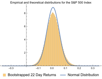
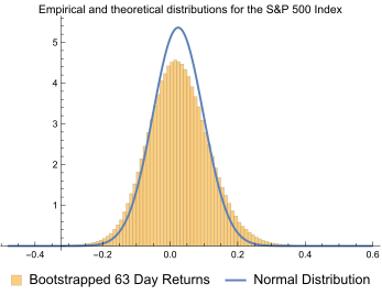
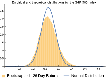
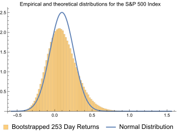
The best distribution then, for practical purposes, is to bootstrap market data to create an empirical distribution. When we do this, and compare the result to what would be obtained from a normal distribution that has the same mean and standard deviation, we can immediately see that the empirical distribution is leptokurtotic: it has fewer minor events than the normal distribution, and has many more major events than the normal distribution. As previously mentioned, the entire return of any investment is almost always driven by its tails: large infrequent events. If we use the normal distribution, we are grossly mismeasuring the tails. At a minimum, this means that we are substantially underestimating the risks involved. It also means that any results that are sensitive to the use of normal distribution dependent statistics such as the standard deviation, are highly suspect and most likely wrong. And that means that the entire edifice of modern finance is built on quicksand because the standard deviation is everywhere: it is present in the CAPM, it is present in Black-Scholes, it is present in Modern Portfolio Theory, and so on. The results of this are that we have catastrophic events such as the 2007-2008 financial crisis, the 2000 tech meltdown, the 1997 Long Term Capital Management Crisis, and 1987 stock market crash, and so on, occurring with great regularity.
Figures 1 and 2 are some comparisons of the theoretical distribution (i.e., the normal distribution) versus an empirically derived bootstrapped derivation. As is immediately apparent, regardless of the time frame, the empirical distribution shows substantially more events in its tails (i.e., they're fatter) than the theoretical, and many fewer events in its peak.
The best measure of risk is...
Now that we have a better distribution, what is a good measure of risk with which to replace the standard deviation? The standard deviation has a series of problems: it doesn't measure the impact of a sequence of events, it doesn't capture the tails of a non-normal distribution, and it doesn't psychologically correspond with any practical measure of risk because it does not answer the question, how much could I lose?
There is a measure that captures the tails, captures sequences and answers the question, "how much could I lose"? That measure is the maximum drawdown. A drawdown is simply how much an investment drops from its peak. If an investment was worth $80, then $90, then $100, then dropped to $85, then $80 and then $75, and then turned back up again, the drawdown would be $100 (the peak) - $75 (the subsequent trough) divided by $100 or $25/$100 = 25%. A maximum drawdown is simply the highest of all the measured drawdowns.
This measure explicitly incorporates the effects of sequences, is affected by tail events, handles non-normal distributions with aplomb, and also answers: "how much could I lose?"It represents what would happen to the unluckiest possible investor: one that got in at the exact highest price, waited until the the price fell to its exact lowest, and then got out.
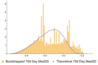
This is a measure that has been well known to futures traders but not to other market participants and deserves to be broadly adopted. Figure 3 shows the empirically derived frequency of maximum drawdowns versus the theoretical frequency. Yet again, the theoretically derived maximum drawdowns are wrong. The theoretical distribution overstates the frequency of small drawdowns and understates the frequency of larger ones. Additionally, sampling via the normal distribution does not preserve the autocorrelation structure present in any investment. Figure 3b shows the maximum drawdown distribution when sampling
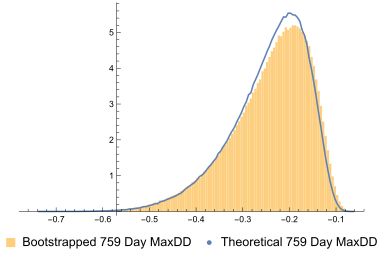
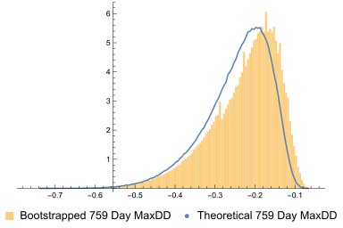
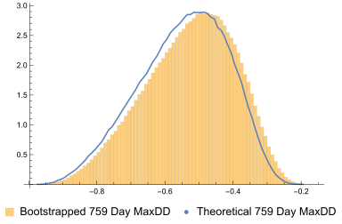
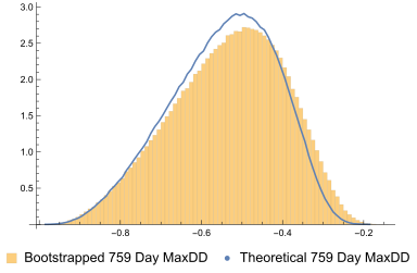
Since the maximum drawdown is the statistic that shows you the maximum expected loss you might have in a given investment, these over and understatements that result from the assumption of normality are very dangerous. Furthermore, these examples are for a very diversified capitalization weighted index. If there is anywhere that a normal distribution should work, it should be there. But even here it doesn't work. When we extend this analysis to other indexes, and then to individual stocks, we find that the normal distribution gets worse and worse. Figure 4 shows the maximum drawdown distributions sampling 1, 10 and 100 days at a time respectively for Intuitive Surgical (ISRG). As is immediately apparent, the correlation structure really matters and, yet again, the normal distribution doesn't properly reflect the characteristics of ISRG.
Conclusion
The assumption of the normal distribution is embedded everywhere in finance. It appears explicitly, in the form of assuming the normal distribution, and implicitly, in the form of metrics such as the standard deviation. Unfortunately, as we can see above, this assumption is wrong, and produces answers that are incorrect. Markets are inherently unstable, a fact that needs to be recognized in financial modeling. This is particularly important when building models such as the CAPM and Modern Portfolio Theory that include an explicit risk-return tradeoff. The lack of an understanding of this fact also produces the famous "volatility smile"in options prices: the smile occurs because the market understands that it is not driven by a process with a normal distribution. This incorrect assumption also drives much of VaR based analysis and the methods typically used to rate investment managers (e.g. the Sharpe Ratio). Either these models need to be rebuilt with distributions and statistics that are empirically derived, or they need to be rebuilt with theoretical distributions that, while not normal, capture the autocorrelation and fat tailed aspects of the markets. In addition, there are also cross-correlation/covariance relationships between assets that must be considered: empirical distributions can handle these naturally (by preserving the relationships while sampling) but theoretical distributions cannot without lots of extra mathematical machinery, and, in most cases, a large number of dubious assumptions.
Footnotes
-
Or variance. For purposes of this argument, the two are equivalent since the standard deviation is simply the square root of the variance. ↩
-
Normal distributions will overstate the return and understate the risk. ↩
-
https://jurnalilmiahmanajemen.files.wordpress.com/2011/03/stock-price-overreaction-effect.pdf ↩
-
Technically it uses the lognormal distribution, but that is a distinction without a difference since continuously compounded normally distributed returns create lognormally distributed prices. ↩
-
What happens if you miss the best days in the Stock Market? ↩
-
See “The best distribution is an empirical distribution” for examples of the types of things about which we know nothing. ↩